
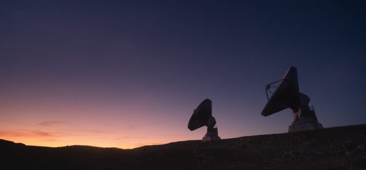
How a software modem turns bytes into sound and the sound back into bytes: the modern signal science, examined through a single VARA FM session.
Every digital mode you run uses a modem: something that turns bytes on one end into a sound a radio can transmit, and turns that sound back into bytes at the far end. The same principle powered the early computer networks that sent data over analog telephone lines. These functions can be performed by a hardware device (TNC), or by software running on a general-purpose computer. Today we are looking at the software modem VARA FM — one of the better ones, and the least documented. It incorporates many of the important techniques used in modern digital communications and because of that it is a great case study for this series.
Before any eyebrows are raised, I’ll acknowledge a couple of well-known issues:
- VARA is a proprietary Windows-only closed-source software, with its higher-speed modes sitting behind a paid license. It doesn’t meet the community’s expectations for the open, interoperable software we would like to see in a hobby centered on experimentation and learning. This criticism, however, would ring hollow coming from somebody who also makes a living selling to ham radio operators. Digirig products are open-source hardware, but physical goods protect a business opportunity far better than software does — releasing the design doesn’t give away the product. My view is that the man put serious knowledge and time into making a software modem that works well and he deserves to be compensated for his work.
- Reflected in the FCC’s rules is the expectation that data on amateur radio bands stays open to inspection. VARA doesn’t encrypt in the traditional sense, but that is not the same as being inspectable. The software doesn’t support a monitoring mode for decoding third-party traffic, and its higher-speed modes sit behind the paywall. This raises the question of whether the software is compliant for use by amateur radio operators in the USA. I’m not going to attempt legal analysis here, but it is worth pointing this out.
- This writeup touches on the details of VARA’s implementation as an academic curiosity and a way to demonstrate the application of signal science in a real-world software modem. I don’t believe it conflicts with VARA’s license agreement. My process for analyzing the modem involved using an AI agent to listen to live VARA sessions, work out their purpose and contents, replay fragments of the audio, and match what it heard against publicly available analysis and existing knowledge in the fields of communications and DSP. Doing this reminded me of the film Project Hail Mary, in which Dr. Ryland Grace teaches the ship’s computer to translate the alien’s language. That said, there is no expectation of the information here being complete or accurate.
This is the first of multiple parts, each covering one layer of a software modem with VARA FM as the case study.
The session
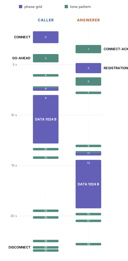
Let’s start with an example of a complete session: here is one entire contact recorded on a single computer running two copies of VARA FM from separate folders, each configured to use its own Digirig, connected with a crossover cable. The whole exchange takes under 22 seconds from the first burst to the last, with 1,024 bytes moved in each direction.
Two kinds of burst
A careful observer will notice that the bursts do not all sound or look alike: at some moments the audio is almost melodic and the waterfall shows a sparse scatter of lines, while at others it is a wall of hiss that fills the band. These are two classes of burst common in communications, and they are the subject of this part; we’ll call them the tone pattern and the phase grid. The two have distinct purposes, and the modem switches between them as the session progresses.
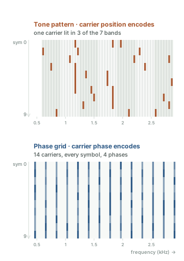
The tone pattern is a kind of pilot signal. Its purpose is to draw the receiving side’s attention and help it prepare for the data that follows. It is conservative with bandwidth and carries little information. Once the receiving side is armed, the phase grid fires up, using as much of the bandwidth as is available to push the payload through as fast as possible.
Both kinds are built from the same raw material. A transmission is a sequence of symbols sent back to back with no gap between them — 24 ms each in a phase grid, a shade shorter (21.3 ms) in a tone pattern — so within a burst there is never an instant without signal. Inside one symbol the modem places tones on a set of evenly spaced frequencies; the ones it lights up are its carriers, and what you hear is all of them sounding together.
The two classes side by side
| Tone pattern | Phase grid | |
|---|---|---|
| Role | acquisition and signaling | payload |
| Family | MFSK — the message is which frequency is active | OFDM — the message rides in each carrier’s phase (and, at higher speeds, its amplitude) |
| Information | a few bits, by carrier position | up to 8 bits on every carrier in use |
| Bandwidth | 3 carriers out of 49 (600–2,860 Hz) | the whole channel — 58 in narrow (470–3,140 Hz), up to 116 in wide (280–5,670 Hz) |
| Symbol duration | 21.3 ms (no guard) | 24 ms (21.3 ms body + ⅛ guard) |
| Receiver needs | an energy detector | symbol timing, a phase reference and error correction |
| Error correction | none; redundancy from repetition and diversity | a rate-1/2 turbo code |
| Failure mode | the detection vote falls short | the checksum fails after decoding |
| Trade-off | robust and cheap to detect, but a very low rate | a high rate, but needs a clean channel |
| First used | the “Piccolo” diplomatic radiotelegraph, 1962; touch-tone dialling a year later | the Collins Kineplex radio modem, 1957; mass use came with DSL |
| Also seen in | FT8, WSPR; Wi-Fi and LTE use similarly sparse preambles for acquisition | 802.11, DVB-T, DAB, LTE and 5G payload; VDSL |
| In VARA | burst detection, addressing, acknowledgements and control frames | all payload, the connect request, the CQFRAME beacon |
Where the numbers come from
Now hold on to your hats, there will be some theory and math involved, I’ll try to keep it simple.
Each of the carriers could take very little bandwidth if they remained a continuous tone. We can see this kind of spectral purity if we look at the mains 50/60 Hz hum or if you fall asleep on your CW key. There is no information in it though. If we want to send data we need to change one or more of the signal’s characteristics: frequency, amplitude, or phase. This spreads what otherwise would be a narrow line of the spectrum. The faster we change the signal, the more bandwidth it consumes. This is the reason why the edges of CW tones are faded in and out by the modern transceivers to reduce the spectral splat.
With information consuming bandwidth, there is a theoretical ceiling on how much error-free data a channel can carry. The Shannon–Hartley theorem pins that ceiling to just two things: the channel’s bandwidth and its signal-to-noise ratio — and, notably, not to how we slice the channel into carriers. These are two ends of one knob: pack the carriers tightly and each symbol has to become longer, shorten the symbols and the carriers have to be spread out — one is simply the reciprocal of the other. Neither end moves the ceiling, so the number of carriers is not a lever on speed at all — it is chosen for something else entirely.
The carrier count is chosen for robustness and there are good reasons to stay away from the extremes: Too few carriers, and a single narrowband whistle — a birdie, a heterodyne — wipes out a large portion of the signal; you want enough that any one interferer costs only a sliver. Too many, and they crowd so close that the ordinary frequency wobble of a real radio or Doppler effect smears each carrier into its neighbors.
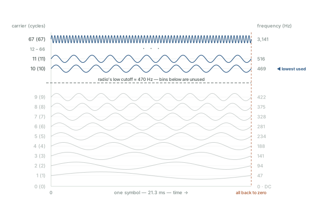
The sweet spot for the carrier spacing is between 40 and 90 Hz, and VARA settles at 46.875 Hz. How many carriers that yields depends on how much of the audio band the mode is allowed to fill. A narrow FM channel gives about 3 kHz to work with, and its bottom edge is off-limits: the lowest slot is DC, and the few hundred hertz above it fall in the sub-audible tone-squelch region our radios roll off. So VARA skips the lowest ten slots and lights carriers 10 through 67, the highest landing at 3,140.6 Hz — 58 carriers in all, and they are the ones that carry the data.
Well within the efficiency target, the choice of 46.875 Hz however seems odd. As you can imagine it’s not incidental and the reason for it is computational efficiency. The typical soundcard samples the audio at 48 kHz. For efficient processing, a modem running on a binary computer works with a transform size that is a power of two. The transform size is chosen to be 1,024 points, which is a power of two and a round number for processing. This choice leads to the carrier spacing of 48,000 ÷ 1,024 = 46.875 Hz, which is nearly perfect for the robustness argument.
That same transform also sets how many carrier slots exist at all. The modem lays out a grid of 128 of them in the transform’s lowest bins, reaching to about 6 kHz. Narrow FM uses only the lower part of that grid — the 58 we just counted — while VARA’s wide modes open the throttle and climb much higher, filling as many as 116 carriers near 5.7 kHz. The number sounding at once is a property of the mode; the grid behind them, and its 46.875 Hz spacing, are not.
The symbol length is then not a separate decision. For the carriers to stay independent — the property that lets them sit side by side without interfering — each must fit a whole number of cycles into one symbol, which forces the symbol to last exactly the reciprocal of the spacing: 1 ÷ 46.875 Hz = 21.3 ms. The spacing and the symbol length are one choice seen from two sides. In phase grid VARA then prepends a short guard interval, an extra eighth, so each symbol can survive a little echo — bringing the transmitted symbol to 24 ms and the modem to about 42 symbols a second. The guard is not used in tone pattern, which is a little more robust to echoes and multipath.
What’s next
That wraps up the quick overview of the two kinds of burst — in data transmission generally, and in VARA specifically. In the next part we’ll take a deep dive into the tone pattern — the simpler of the two — and see how it works, what information it carries, and how VARA encodes and detects it.
I encourage feedback on the series and welcome questions, corrections and criticism. The comments section is open below.